1 Introduction
Recent work, under the umbrella title of Singular Learning Theory, seeks to better understand questions of large model interpretability and training dynamics via the geometry of the loss landscape. The central object of the study is the posterior distribution on weight space.
Take a parameter space \(W\), whose points \(w\) each describe a function, a prior distribution \(\phi\) on \(W\), and a dataset \(\mathcal{D}_n\) of \(n\) input output pairs \((x_i, y_i)\). The probability that a parameter \(w\) describes the data generating function, after observing \(\mathcal{D}_n\) is given by the posterior distribution:
Accurate and efficient sampling from this distribution fundamentally underlies all work in singular learning theory for interpretability and steering.
The Local Learning Coefficient, a complexity measure, is approximated via an expectation over such a distribution, and susceptibilities, used in interpretability (Lau et al., 2025; Baker et al., 2025; Gordon et al., 2026) and in patterning (Wang & Murfet, 2026), are similarly defined as covariances over the posterior. In all cases, it is infeasible to compute the integrals involved in these expectations, and they are instead approximated using a set of samples from the posterior distribution.
As such, establishing the accuracy of this sampling process is critical to current and future development of this agenda. Previous work in this direction has studied the accuracy of sampling methods in contexts where the underlying distribution is well understood (Xu, 2024; Hitchcock & Hoogland, 2025).
In contrast, we present a test for measuring the quality of a sampling method in a situation where the posterior distribution is almost entirely unknown. Rather than benchmark techniques against a ground truth, we rely on the following heuristic:
In this paper we examine several methods of sampling from the posterior of a large language model. We also assemble a selection of probe tasks, sets of contexts which are grouped into two classes by whether they exhibit a particular phenomenon. (For example, a set of contexts that are all names of historical individuals, grouped by whether or not the individual is American.)
For each probe and method, we collect losses on the probe contexts for a set of samples generated by that method. If the sampling method is effective, we hypothesize that the information we collect will allow for stronger performance on a predictive classification task.
2 Previous Work
2.1 The Local Learning Coefficient and SGLD
Prior work on sampling in singular learning theory has focused primarily on estimating the Local Learning Coefficient (LLC) (Lau et al., 2025). The LLC \(\lambda(w_0)\) is a measure of model complexity around a local minimum \(w_0\) in parameter space. It is estimated from expectations over a localized, tempered posterior
a more specific form of Equation 1. Here \(L_n\) is the empirical loss over a dataset \(\mathcal{D}_n\) of size \(n\) and \(\beta > 0\) is an inverse temperature. The first term is a Gaussian prior centered at \(w_0\) with variance controlled by a localization strength \(\gamma\); the second term concentrates the distribution on nearby parameters with low loss. Given samples from \(p\), the LLC is estimated as
See (Watanabe, 2013; Lau et al., 2025; Hitchcock & Hoogland, 2025) for a derivation as well as a more detailed discussion of the properties of this estimator. Practical estimation therefore hinges on drawing good samples from \(p\) at large \(n\).
The primary method for achieving this has been Stochastic Gradient Langevin Dynamics (Welling & Teh, 2011), a Markov chain Monte Carlo method described in further detail in Section 3.1.
2.2 Assessing Sampling Quality
There are several ways of assessing the quality and correctness of sampling in singular learning theory, and it is helpful to distinguish between them.
At a basic level, one can study whether sampling is converging at all by looking at the statistical properties of the sampling Markov chains. This involves statistical tests for whether individual chains are converging, whether multiple chains appear to be converging to the same thing, and how correlated draws are within a chain. See, for example, Gelman & Rubin (1992); Geweke (1992); Brooks & Gelman (1998); Vehtari et al. (2021), and Hitchcock et al. (2026) for how these are applied to LLC and susceptibility estimation in practice. These diagnostics do not attempt to assess whether sampling is converging to the correct thing, only whether sampling is converging to something.
Assessing whether sampling is converging to the correct distribution can be done in special cases where we have sufficient understanding of the target posterior distribution. In deep linear networks (DLNs), neural networks without activation functions, certain invariants of the target distribution are known due to Aoyagi (2024). Xu (2024), Lau et al. (2025) and Hitchcock & Hoogland (2025) test sampling methods in DLNs by evaluating how well such invariants can be recovered.
When we don’t have ground truth information about the target distribution, such as in large language models, the situation is much more difficult. In the Bayesian deep learning literature, methods are often assessed on the basis of predictive performance. This is an accessible metric which is often relevant to downstream applications, but conflates representation of the posterior distribution (which we aim to sample from) with representation of the predictive distribution. In the extreme case, the sampler can collapse structure in the posterior down to a single point where the likelihood is maximized while achieving optimal predictive performance, perhaps better than the ‘true’ predictive distribution.
In this work, we propose to assess sample quality by looking at how much semantic information about the data distribution is retained in samples from the posterior. This is based on the work of Baker et al. (2025); Gordon et al. (2026); Kreer et al. (2025); Adam et al. (2025); Murfet et al. (2026) which demonstrate that quantities like susceptibilities and Bayesian influence functions (BIF) , estimated via posterior expectations , yield interpretable insights into how a large language model generalizes semantic relationships across different inputs. We do this by looking at the predictive performance of probes (small classifiers) trained directly on a quantity closely related to a BIF.
Because the BIF is an expectation over the posterior, a sampler which fails to capture structure in the posterior which is relevant to the probing task will not produce probes which perform well, which is in contrast to assessments via predictive performance of the LLM itself. Hence our key heuristic: An interpretability method that is derived from an approximation of the posterior can be reversed and used to study the quality of that approximation.
2.3 Testing Sampling with an Unknown Posterior
We design and implement a test that measures sampling correctness without assuming known structure in the posterior. Both susceptibilities and BIFs aggregate and process losses for a fixed set of data points over parameters sampled from a Markov process approximating the posterior distribution on weights. They observe that similar data points can be identified via data encoded in these loss traces. Loss traces collected via sampling, and no other labeling, are robust enough to identify, for example, conjugations of the same base verb, or a variety of synonyms for groups of people.
These interpretability methods can capture rich structure. We believe that this structure is a direct result of capturing details of the posterior distribution. To test this, we can compare multiple procedures for approximating samples, some of which are known to be worse than others, and verify the key heuristic directly.
The unsupervised feature detection used in (Baker et al., 2025; Gordon et al., 2026; Murfet et al., 2026) is not well suited to this sort of comparative analysis, (though see Appendix H of (Gordon et al., 2026) for some analysis). We previously identified thousands of susceptibility clusters, but the number of clusters as well as inherent randomness in the clustering algorithm made sets of clusters found via different methods difficult to compare.
In the current work, we replace feature detection with probes, which allows for a much more concrete comparison.
3 Methodology
3.1 SGLD Sampling
Here, we provide an overview of Stochastic Gradient Langevin Dynamics and the details of our implementations. See Appendix A for a more thorough description.
SGLD produces a sequence of points \(\{w_i\}\) in parameter space, generated by a Markov chain. Markov chain methods in general work by constructing a kernel distribution \(\mathcal{K}(w, -)\) which describes the probability distribution over the space of parameters if you start at \(w\) and make a single update step. The kernel distributions are easily computed, so it is tractable to start at an arbitrary \(w_0\), select \(w_1 \sim \mathcal{K}(w_0, -)\), and repeat the process several times. However the kernel is designed so that the \(N\)-step distribution \(\mathcal{K}^N(w_0, -)\), the probability distribution describing where \(w_N\) will be, becomes extremely similar to the target distribution for \(N\) large, regardless of the initial choice of \(w_0\).
We write our target distribution as an update step by describing a vector that we add to \(w_t\), though the vector added has its entries described by a random variable.
The update step for the tempered posterior in SGLD is given by
The update step can be understood as a sum of three components
- The localization \(-\frac{\epsilon}{2}\gamma (w_t-w_0)\) is a vector pointing towards \(w_0\). Localization keeps the chain from moving too far away from a given small region. Setting \(\gamma\) large results in chains that stay closer to \(w_0\).
The gradient term \(- \frac{\epsilon}{2} n\beta \nabla_{w} L_m(w_t)\) is a vector pointing in the direction from \(w_t\) that minimizes (minibatch) loss. This is a slight difference from the formula in section 2.1. We pin the number of samples used for loss to a fixed \(m\) independent of \(n\beta\) for computational efficiency. Since \(n\) and \(\beta\) only enter this formula as a pair, we now regard \(n\beta\) as a single inverse temperature parameter.
When \(n\beta\) is large, the Markov process is more sensitive to the loss landscape. When \(n\beta\) is zero, the sampling process does not use gradient information, and its stationary distribution is a Gaussian centered at \(w_0\).
- The noise \(\sqrt{\epsilon}\, \eta_t\). Here \(\eta_t\) is a random variable sampled from a Gaussian with identity covariance. This term causes the chain to move randomly through parameter space. The step size \(\epsilon\) cannot be independently adjusted, it also controls the size of the other two terms.
The effect of these terms together is to generate a chain that moves randomly through state space, but is constrained to stay close to \(w_0\) and favor parameters with lower loss. The discrete time process described by this Markov chain is a discretization of a continuous time process whose stationary distribution is the desired posterior. So for small \(\epsilon\) the Markov chain hopefully approximates the distribution closely.
3.2 Loss Traces
General loss traces are an artifact produced during sampling that record the average loss at each step of the Markov process. They are a useful tool in understanding the sampling process. Note that the minibatch loss used at each step is not the same, though for sufficiently large \(m\) we can hope that \(L_m\) is a reasonable approximation of population loss.
Given a sequence \(\{w_i\}\) of \(N\) points in parameter space produced by SGLD and a specific data point, which in the case of a language model means a token \(y\) immediately following a context \(x\), the token loss trace is the length \(N\) vector \([ \ell_{x,y}(w_0),\dots, \ell_{x,y}(w_{N-1})]\) recording the loss at each point of the specific task of predicting \(y\) after \(x\).
3.3 Probes
A probing task is a set \(C:= \{c_i\}\) of contexts as well as a labeling function \(s: C \to \{0,1\}\). For our purposes the set of contexts is from a narrow domain, and the labeling function detects specific qualities in the text. For instance, \(C\) could be a set of movie reviews, and \(s(c) = 0\) if the review \(c\) is favorable and 1 if the review is unfavorable.
| Context | Group |
|---|---|
Q: What do carnivores eat?A: animals | 1 |
Q: What color is neptune?A: yellow | 0 |
Q: Which carbohydrate is produced by photosynthesis?A: glucose | 1 |
Q: Where does mechanical digestion begin?A: intestines | 0 |
sciq-tf probing task. Each context is a science-exam question paired with a candidate answer; the group label is 1 when the answer is correct and 0 when it is not. The newline is part of the context.We used a collection of twenty one different probing tasks, covering a range of difficulties and areas, as listed in Appendix B.
3.4 Measuring Probe Performance
A feature function is a mapping \(f:C\to \mathbb{R}^k\). We can evaluate a feature function by its ability to separate the different groups of a probing task. Specifically, we investigate how well \(s(c)\) can be determined if we know the value of \(f(c)\).
To do this we decompose the set \(C\) into \(C^{\text{train}} \sqcup C^{\text{val}} \sqcup C^{\text{test}}\), a random partition into subsets containing 70%, 15% and 15% of the total contexts.
Then we use the features \(f(C^{\text{train}})\) and their corresponding labels given by \(s\) to train a model which predicts \(s(c)\) given \(f(c)\). The model is a function \(m_\theta: \mathbb{R}^k \to [0,1]\) which is trained to minimize prediction error
with the addition of some regularizers that depend on the specific model.
We looked at a few different choices for feature vector and model. Most experiments used as features last token loss traces, as well as loss traces averaged over the context. For these feature sets, we used logistic regression models, as well as shallow multi-layer perceptrons.
In addition, we considered using the concatenated loss traces for all tokens in a context, and having as a model a small multi-headed transformer capable of processing feature vectors of different lengths.
Given a model trained on \(C^{\text{train}}\), we evaluate it on a secondary dataset using Area Under the Receiver Operating Characteristic curve, or AUROC. The AUROC score for a model \(m_\theta\) and a set of contexts \(D\) is
To avoid overfitting during training as well as hyperparameter and architecture selection for the models, for each probe task and choice of feature function, we swept over a grid of choices for hyperparameters, and for each choice \(\alpha\) of hyperparameters, trained a model \(m_{\theta_\alpha}\). Then we selected as our model the one which maximized AUROC on the validation set \(C^{\text{val}}\). We then recorded the AUROC of this choice on \(C^{\text{test}}\).
3.5 Loss Traces as Features
We chose to use features derived from these per token loss traces due to previous work on Bayesian Influence Functions. Kreer et al. (2025); Adam et al. (2025) have shown that the influence function kernel created by taking dot products between such loss traces thought of as vectors captures interesting high-level abstractions about the text. Analysis on the columns of this kernel matrix has identified synonymous word pairs, shared meaning across language, and abstract concepts like goals in models as large as 3 billion parameters.
The columns of the BIF kernel are produced from linear maps applied to (normalized) loss traces, so little is lost from using the loss traces themselves as our feature vectors. Based on what has previously been found, we expect that a probe trained on token loss trace vectors should also capture high-level features in the contexts.
Before fitting a probe, we standardize each feature coordinate using the mean and standard deviation computed on \(C^{\text{train}}\). The same transformation is then applied to \(C^{\text{val}}\) and \(C^{\text{test}}\), avoiding leakage from the held-out sets.
We wish to emphasize that we are interested in directional change, not overall performance on the probe. We do not study any feature sets or models that produce near optimal AUROC values on our probing tasks. Rather, among feature sets derived from sampling and otherwise comparable, an observed difference in AUROC scores for any class of model is evidence that one set of samples has captured more meaningful variations in the posterior.
4 Results
For Qwen 2.5 3B we studied SGLD sampling with a range of different hyperparameters for various probes.
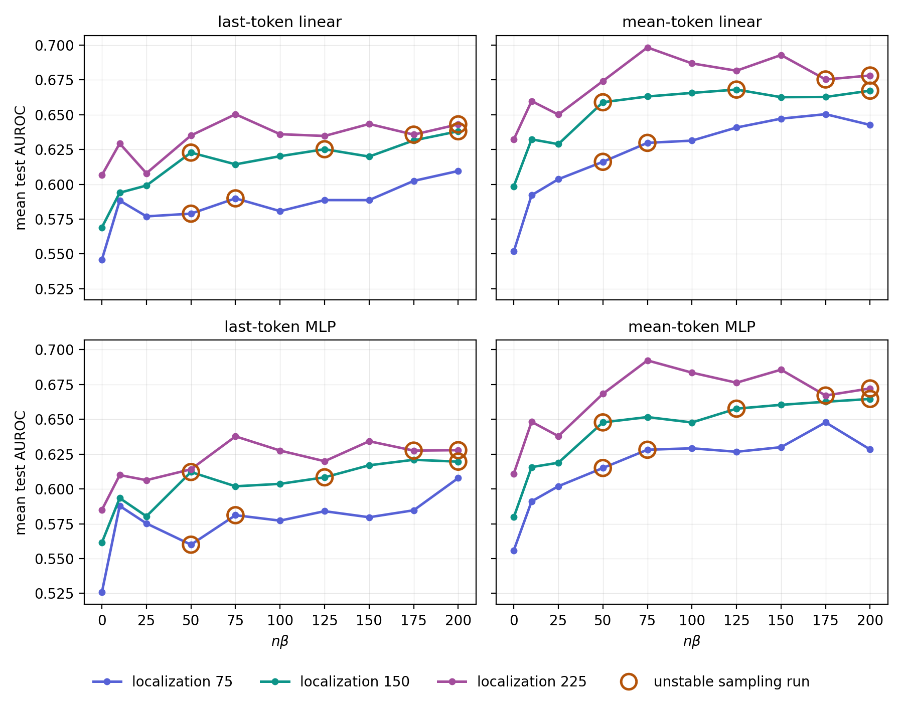
Following the notation of equation 5, we used a step size of \(\epsilon = 5e{-}05\) and swept over a grid of thirty values for localization and \(n\beta\) parametrized by
We identified two trends, that persisted across all probe architectures studied.
Probe performance increases with \(n\beta\). For localization 75 and 150, we see a near monotonic improvement in average probe performance as \(n\beta\) increases, validating our belief that SGLD is successfully incorporating gradient information to explore more interesting regions of the loss landscape around \(w_0\). At localization 225, the data show an increase in average probe performance, followed by a plateau.
For every fixed probe architecture and localization, setting \(n\beta=0\), the equivalent of sampling from an isotropic Gaussian at the starting point, underperforms every other possible value.
Probe performance increases with \(\gamma\) For every fixed probe architecture and value for \(n\beta\), increasing localization results in a monotonic improvement in probe performance. This is expected, considering Lau et al. (2025), which gives a theoretical definition of the LLC based on variations in the posterior in an extremely small neighborhood of \(w_0\).
4.1 Individual Probe Tasks
The trends we observe above are presented in the aggregate, but detailed analysis of individual probes reveals these patterns are robust to many settings. We present the full data in Figure 2, and highlight some key points here
A few probing tasks were too difficult for any set up. Of the 21 probing tasks studied, 5 had no choice of architecture or hyperparameters that achieved an AUROC above 0.6. Removing these probing tasks from the average does not change results.
Individual probe task results largely reflect aggregate results The aggregate-best hyperparameter setting (localization 225 and \(n\beta\) 75) ranks in the top 5 of 30 for 11–12 of 16 individual tasks, and in the top 10 for 15 of 16, in every architecture.
View the plotted values as a table
4.2 Loss Chain Dynamics
Of the thirty choices of hyperparameters in each plot of Figure 1, seven are flagged as unstable. As described in Appendix A.2, the loss traces used in a probe were computed from two independent chains. A trace was labeled unstable if the general loss traces (Subsection 3.2) for two chains did not approximately agree, or either general loss trace showed large drift during the window when per token loss traces were collected.
We observe that despite loss traces indicating that a sampling process had not properly converged to a stationary distribution, the mean AUROC scores do not identify these points as outliers. This is a limitation of the method, and emphasizes that any test of sampling quality based on probe performance cannot replace more common tests for convergence. In Figure 3 we present the plots of the loss traces with further analysis.
5 Limitations and Future Work
Though probes can measure and validate sampling methods, they can only ever be a single tool. There is considerable risk in benchmarking sampling results primarily or exclusively by probe performance. Scores on probing tasks indicate nothing explicitly about the correctness or stability of a sampling procedure, and the heuristic that improved performance on probes comes from improved accuracy in posterior approximation is likely false when pushed to the extreme. There is substantial risk of overfitting if sampling methodologies are optimized around performance on a few probes.
Further, while probing can validate a sampling technique, it cannot as of yet produce insights into the probe task that are better than other methods. In particular, the loss trace probes discussed above all underperform probes based in activations. This is not surprising, residual stream activations are a richer object from an information theory context and also much higher dimensional.
▶Appendix A
SGLD Details
A.1 Preconditioner
In this appendix we present our algorithm for SGLD in more complete detail. Recall the formula for the update step given above:
For the results collected above, we used a preconditioned variant of SGLD, following Li et al. (2016), whose update step is given by
\(G_t\) is a diagonal preconditioner with formula given by
for \(V_t\) an exponential moving average of the magnitude of the gradient which is updated at every step via
The preconditioner scales the coordinates of the update step, such that update steps in coordinates where the gradient term is large (as determined by an exponential moving average) are shrunk relative to coordinates where the gradient is small. The preconditioner is designed to produce more even rates of mixing across parameters which see different magnitudes of gradient updates.
Note that \(V_t\) is computed from the raw minibatch gradient \(\nabla_{w} L_m(w_t)\) rather than the tempered gradient \(n\beta\nabla_{w} L_m(w_t)\), so \(n\beta\) does not enter the update formula, which enters the dynamics only as an overall multiplier on the loss-gradient drift.
A.2 Drawing Parameters
For each choice of hyperparameters, we generated per token loss traces by first taking 12,000 burn in steps, and then recording the loss on the probe task contexts at 250 different points, each separated by 40 steps of the Markov chain to increase effective sample size.
We generated two independent chains for every set of hyperparameters, resulting in 500 dimensional feature vectors for each probe task.
▶Appendix B
Probe Tasks
For probe tasks, we chose a selection of probes that covered a diverse range of topic and difficulty. Our primary source for probe datasets was Kantamneni et al. (2025), though we noted several duplicate prompts in the datasets there, which needed to be removed. Below is a full list of the probes we used as well as citations for the original data
target column.| Dataset | Source | Contexts and groups |
|---|---|---|
| hist-fig-ismale | Gurnee & Tegmark (2024) | Contexts are bare names of historical figures. Groups: female (g0) vs. male (g1). |
| hist-fig-isamerican | Gurnee & Tegmark (2024) | Contexts are bare names of historical figures. Groups: non-American (g0) vs. American (g1). |
| headline-isobama | Gurnee & Tegmark (2024) | Contexts are New York Times headlines. Groups: headlines about Barack Obama (g1) vs. headlines that are not (g0). |
| sciq-tf | Welbl et al. (2017) | Contexts are “Q: … A: …” pairs built from SciQ science-exam questions. Groups: the stated answer is incorrect (g0) vs. correct (g1). |
| just-is | Hendrycks et al. (2021) | Contexts are first-person scenarios asserting a desert or expectation claim, from the ETHICS justice subset. Groups: claim judged unjustified (g0) vs. justified (g1). |
| high-school | Gurnee et al. (2023) | Contexts are natural-text snippets ending at an occurrence of “high”/“school”. Groups: the snippet ends with the compound “high school” (g1) vs. another use of the constituent words (g0). |
| glue-sst2 | Wang et al. (2019) | Contexts are movie-review sentences from SST-2. Groups: negative (g0) vs. positive (g1) sentiment. |
| spam-is | Team AI & Ishii (2017) | Contexts are SMS text messages. Groups: ham (g0) vs. spam (g1). |
| us-timezone-los-angeles | Gurnee & Tegmark (2024) | Contexts are bare US place names. Groups: place outside (g0) vs. inside (g1) the Los Angeles (Pacific) time zone. |
| arith-mc-a | Allen Institute for AI (2024) | Contexts are arithmetic multiple-choice problems with options A–D, always ending in “Answer: A”. Groups: A is the wrong (g0) vs. the right (g1) answer. |
| news-class-politics | Dublish (2024) | Contexts are news snippets (headline plus lede). Groups: article about politics (g1) vs. other topics (g0). |
| disease-class-digestive | Kasaraneni (2019) | Contexts are medical-paper abstracts describing diseases. Groups: digestive-system diseases (g1) vs. other disease categories (g0). |
| twt-emotion-sadness | Gupta (2021) | Contexts are tweets. Groups: tweets expressing sadness (g1) vs. other emotions (g0). |
| circa | Louis et al. (2020) | Contexts are “Q: … A: …” pairs where the answer is an indirect response to a yes/no question. Groups: the answer means no (0) vs. yes (1). |
| codexglue-defect-qemu-max128 | Zhou et al. (2019) | Contexts are C functions (≤128 tokens) from the qemu project, from the Devign/CodeXGLUE defect data. Groups: secure (0) vs. vulnerable (1). |
| codenet-re-python-max128 | Puri et al. (2021) | Contexts are short Python competitive-programming submissions (≤128 tokens) from IBM Project CodeNet. Groups: runs correctly, i.e. Accepted (0), vs. Runtime Error (1). |
| ethics-commonsense | Hendrycks et al. (2021) | Contexts are short first-person moral scenarios from the ETHICS commonsense subset. Groups: morally acceptable (0) vs. morally wrong (1). |
| politeness-wiki-max64 | Danescu-Niculescu-Mizil et al. (2013) | Contexts are standalone Wikipedia editor talk-page requests (≤64 tokens). Groups: bottom politeness quartile, impolite (0), vs. top quartile, polite (1). |
| politeness-stack-max64 | Danescu-Niculescu-Mizil et al. (2013) | Contexts are standalone Stack Exchange requests (≤64 tokens). Groups: impolite (0) vs. polite (1), as above. |
| sarc-chain1-paired-max64 | Khodak et al. (2018) | Contexts are a Reddit submission title plus a top-level reply (≤64 tokens), with each submission contributing both one sarcastic and one non-sarcastic reply (minimal pairs). Groups: not sarcastic (0) vs. sarcastic (1), by the author’s /s self-tag. |
| sarc-chain1-unique-max64 | Khodak et al. (2018) | Same construction, but with a single randomly chosen reply per submission so no context repeats. Groups: not sarcastic (0) vs. sarcastic (1). |